
The difference between deep learning and machine learning depth: the training and adjustment of deep learning
In recent years, deep learning has emerged as a method of fire in machine learning, but compared with non-deep learning machine learning (I attribute deep learning to the field of machine learning), there are still a few big points. The difference is, in particular, the following:
1, deep learning, as the name suggests, the network has become deeper, which means that this deep learning class network may have more layers, what does this mean? That is to say, this deep network needs to learn more parameters. Although we know that there are techniques such as sharing parameters in CNN, under this premise, it may be considered that as the number of network layers increases, the parameters that need to be learned are also Increase, then the problem is coming again, what is the problem with the increase in parameters? Of course, there is a problem. This is the most common problem we have discussed in the field of machine learning, because our purpose is to reduce the generalization error and improve the generalization ability of the model. At this point, it is obvious that deep learning is more general than The machine learning model is complex, and the complex model is not properly trained. As we know, the generalization ability of the model will be significantly reduced.
2. Deep learning is more complicated than the general machine learning model, not only in the model itself (referring to layers and parameters), but also in different working principles. Deep learning no longer requires manual design of specified features. The characteristics of classification are learned by the model itself. This means that deep learning requires more data, which is different from machine learning in general. . For example, the same is to identify the vehicle, Haar-like+Adaboost may only need 2-3k training set, but for deep learning, it may need 20-30k data set, of course, so much data itself matches the model. However, in a general sense, it may be considered that deep learning requires more data (this article does not explore the relationship between big data and deep learning (artificial intelligence), only in the general sense).
In summary, in fact, we have realized the essence of deep learning, in fact, it is very simple, that is, data and models, the two complement each other and promote each other. Recognizing the difference between the nature of deep learning and machine learning in the general sense, you can understand how important the skills and suggestions of arranging and training are for deep learning. It is no exaggeration to say that it directly affects what we just talked about. The generalization ability of the model, and the root cause.
From the sequence of our process of preparing the data set to training to the ideal model, we divide it into the following sections.
1, Data augmentaTIon (data enhancement).
Personal understanding of data enhancement is mainly in the preparation of the data set, because the required data is more and can not be met, you can pass the color (color), scale (scale), crop (crop), flip (Flip), add noise (Noise), Rotation (RotaTIon), etc., this increases the number of data sets, and solves the problem of insufficient data. In recent years, the research on GAN model has also made great progress, and its main starting point is to solve it. Supervised learning of insufficient data, often used for virtual scene simulation, etc., interested can be studied in depth.
2. Pre-processing.
Personally understand that after having the data, can you make good use of this data? How to evaluate the quality of these data? That is to pre-process the data, the premise of pre-processing is to correctly understand the data. Is there a correlation between the data? Suppose you use data augmentaTIon, obviously the correlation between the data sets is larger, say straightforward, you use two identical data in the training set, what is the significance? So the data preprocessing that will be discussed next is very important. Commonly used methods are: normalizaTIon (normalization), PCA (principal component analysis), Whitening (whitening) and so on.
(1) Normalization. It can be said that normalization is mainly doing the same thing: changing the data from a general distribution to a distribution of 0 mean and unit variance. Why do you do this? The reason is that it is easier to converge, this method is commonly used in the Caffe framework (mean value or mean binaryproto file). Batch Normalization (BN) is an upgraded version. The author mainly considers that when a saturated activation function is used, for example, the sigmoid function becomes 0 mean, and the unit variance appears in the approximate linear phase of the function. This is very bad. The middle linear part has the worst fitting ability, thus reducing the model's expression capacity, so BN came into being. Experiments show that the effect sigmoid function is better than the Relu function.
(2) PCA. Study how to condense many original variable information into a few dimensions with the least amount of information loss, the so-called principal component. Firstly, the covariance matrix is ​​calculated, then the eigenvectors of the covariance matrix are obtained, and the original features are linearly transformed to achieve dimensionality reduction.
(3) Whitening. The correlation between the features in the feature vector is removed, while ensuring that the variance of each feature is consistent. Let the eigenvectors X = (X1, X2, X3), for the vector X, the corresponding covariance matrix (estimated from the existing data set) can be calculated. We want the covariance matrix to be a diagonal matrix, because this means that each element of X is unrelated, but our data does not have this property. To understand the coupled data, we need to perform a transformation on the original feature vector so that the correlation between the features of the transformed vector Y is zero. Let Σ be the covariance matrix of X, where: ΣΦ=ΦΛ, then each element in Λ is the eigenvalue of the covariance matrix, and each column vector of Φ is the corresponding eigenvector. If the eigenvector is transformed: Y = XΦ = X(Φ1, Φ2, Φ3), then the covariance matrix calculated from the vector Y is a diagonal matrix. The eigenvalue of the diagonal matrix Λ is the variance of each element of Y, which may or may not be the same. If some dimensions of the transformed feature vector are scaled so that each element of Λ is equal, then the whole The process is whitening.
3. Initialization.
After the current two steps are completed, you can consider how the model parameters are initialized. Here is an example. There are seven methods for parameter initialization in Caffe: constant, gaussian, positive_unitball, uniform, xavier, msra, and bilinear. More often used is xavier for weight initialization, and constant for bias initialization.
4. Activation Functions.
The key to deep learning is the activation function, which is equivalent to a series of nonlinear processing units that are superimposed. It is conceivable that this series of superimposed nonlinear processing units can be approximated in principle. Function (this refers to the effect from input to output). Several commonly used activation functions: sigmoid, tanh, and Relu, but we have introduced the saturation activation functions such as sigmoid and tanh that were widely used before. The training effect in the deep network model is often poor because the gradient disappears. The problem, for example, is an example of a sigmoid function. Since the neural network needs to multiply the first derivative of the activation function in the back propagation, it can be forwarded layer by layer, and 0.930=0.042, which is generated. At the two extremes, there appears a gradient disappearance zone as shown in the following figure. Once the gradient is already small, how can I learn? We use the Relu function in Caffe to effectively avoid this problem.
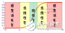
Figure 1: sigmoid function
5. During training (during training).
In the training process, it is necessary to grasp the learning strategy of learning rate. In general, Caffe defines the learning rate in the hyperparameter configuration file (solver.prototxt), and selects the learning rate attenuation strategy (the learning rate is large at the beginning, Then it becomes smaller, how it changes, how it changes, we call it strategy, so we usually talk about it in the paper), and more importantly, you can specify lr_mult to select a layer in the network layer definition. Learning rate, this skill can also prepare for later adjustments. Another very important thing is fine-tune. The use of fine-tuning is usually that you choose a deeper model, which is a more complicated model. You don't need to retrain all the layers, but just train them. Some of the layers, at this point we can stand on the shoulders of the giants (using the weights of the pre-trained model to initialize), can save a lot of work, and more importantly, plus the appropriate tuning will also improve the generalization of the model. Capabilities (because pre-trained models are often not converged).
Specifically, there are several situations:
Pay attention to the name of those layers that need to change the fine-tuning in Caffe (while changing the layer parameters according to their needs, such as the channel of the image, the number of categories of the full-connected layer output, etc.).
6, Regularizations (regularization).
Regularization is also known as Weight-decay. Regularization should be an effective way to avoid over-fitting. Here we insert a analysis of over-fitting. As far as I know, engineers engaged in machine learning often encounter many problems, many bugs, but It can be said that over-fitting is a problem that all engineers must face, and it has strong versatility, which is determined by the method itself. Since everyone will encounter this problem, how can we solve it? Looking back, we said that the essence of deep learning is data and models, and the fundamental way to solve the overfitting must also start from these two directions, then what is overfitting? The image says that you think your model has performed well on the training set, but when you use it on the validation set, the effect is very poor. Further, the data set is too small or the model is too complicated. Obviously it doesn't match. Now we start to analyze from these two directions, two solutions: increase the data set and reduce the complexity of the model (limit the network's capacity). Regularization here is a technique to reduce the complexity of the model. The essence is to control the number of features of the model learning to minimize it, thus preventing the introduction of the sampling error of the training set in the training process. Regularization includes L2. Regularization and L1 regularization.
7, Dropout.
Dropout refers to the temporary discarding of the neural network unit from the network according to a certain probability during the training of the deep learning network, as shown in the following figure. For random gradient descent, each mini-batch is training a different network because it is randomly discarded (for a neural network with N nodes, after dropout, it can be considered as a collection of 2n models), At the same time, each network only sees one training data (each time is a random new network), so that these multiple models are combined, and the average output of each model is used as the result. The Dropout layer is also defined in caffe.
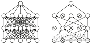
Figure 2 Dropout example
8, Insights from Figures.
If you have done the above method, you still have problems, you need to check it carefully. There are many ways to check it. The most vivid one is the drawing, which is inferred from the figure. . We know that Caffe also provides us with a lot of drawing tools (called visualization), which is quite good for writing papers and scientific research. Closer to home, here are a few pictures from the Internet, these pictures can be drawn from the log through the tools, let us take a look.
Figure 3 shows the loss curve at different learning rates. It is obvious that the four curves in the graph show different performances as the number of iterations increases. The yellow curve decreases first and then increases dramatically as the number of iterations increases. It often causes loss equal to Nan, which is due to the fact that the learning rate of choice is too large (ps: I personally test, there are times when I am modifying some models, the loss is very large, and then choose a larger learning rate, At once, Nan is); the blue curve increases with the number of iterations, the rate of loss reduction is very slow and slow, and the maximum number of iterations set is already large, but the network does not converge, which means that the learning rate is too The green curve decreases with the increase of the number of iterations, and the network convergence is high in a place with a high loss. This shows that the learning rate of the selection is a bit large and has reached the local optimum. Observe to reduce the learning rate when the network loss does not drop; the red curve decreases slowly with the number of iterations, the curve is relatively smooth, and finally converges at a low level of loss. , indicating that the selected learning rate is better. Of course, the figure is an ideal curve, which can only explain the trend of change. In reality, the curve is fluctuating, and there are some burrs (ps: a lot of practice proves that the local optimum and the global optimum are acceptable, that is, red and The process represented by the green curve, of course, most comrades encounter local optimum. At this time, we consider reducing the learning rate on the basis of local optimization and continue training. The difference between the two is that the local optimum will remain in one. On the higher loss, of course, there is no standard for measuring the loss level. Therefore, the local optimum does not mean that the training result is poor. The local optimal result can also be compared with the global optimum because we don't know where the global optimum is.
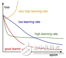
Figure 3: Relationship between learning rate and loss
Figure 4 shows the loss curve of different iterations. It can be seen from the figure that as the number of iterations increases, the change trend of loss is reduced. Note the "width" marked in the figure, if the width of the curve is too Big, it means that the patch you choose is too small, but in fact, the choice of batch is not casually in deep learning, too big, not too good, too small, too big, there will be memory overflow The error is too small. It is possible that a label is difficult to learn. This often leads to the model not converge, or the loss is a mistake such as Nan. At this time, you can use accum_batch_size to solve the problem that you cannot select a larger batch due to lack of hardware.
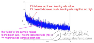
Figure 4: The relationship between the number of iterations and loss
Figure 5 is the accuracy curve of the model on the training set and the verification set. The red curve indicates the classification accuracy of the model on the training set. It can be seen that it is not bad. As the number of iterations increases, the accuracy of the classification increases, and there is a convergence trend; the green curve indicates that the model is on the verification set. The classification accuracy can be seen, compared with the precision of the training set, the gap is very large, indicating that the model is over-fitting, and should be solved by using the solution mentioned above. If there is no big gap between the two and the accuracy is very low, you should increase the capacity of the model to improve performance.
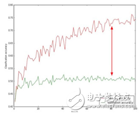
Figure 5: Accuracy curves of the model on the training and validation sets
We are all on the way to the truth.
Power 90W ,output voltage 15-24V, output current Max 6A, 10 dc tips.
We can meet your specific requirement of the products, like label design. The plug type is US/UK/AU/EU. The material of this product is PC+ABS. All condition of our product is 100% brand new. OEM and ODM are available in our company, and you deserve the best service. You can send more details of this product, so that we can offer best service to you!
90W Desktop Adapter,90W Desktop Power Supply,90W Desktop Power Cord , 90W Desktop Power Adapter
Shenzhen Waweis Technology Co., Ltd. , https://www.huaweishiadapter.com