
Take you deeper into the characteristics and applications of the modulator
While many explanations describe modulation as a straightforward multiplication process, the reality is more intricate. For instance, when you apply a signal like Acos and an unmodulated carrier cos(ωt) to an ideal multiplier’s inputs, you essentially create a modulator. This happens because the two periodic waveforms Ascos(ωst) and Accos(ωct) interact at the multiplier's input (assuming a 1V scale factor for simplification), yielding the following output:
\[ V_o(t) = \frac{1}{2} A_s A_c [\cos((\omega_s + \omega_c)t) + \cos((\omega_s - \omega_c)t)] \]
If the carrier Accos(ωct) has an amplitude of 1V (Ac = 1), the equation simplifies further:
\[ V_o(t) = \frac{1}{2} A_s [\cos((\omega_s + \omega_c)t) + \cos((\omega_s - \omega_c)t)] \]
However, in practice, a modulator often performs this function more effectively than a multiplier. A modulator (also referred to as a mixer when altering frequency) is closely related to a multiplier.
The multiplier’s output is simply the instantaneous product of its inputs, while the modulator’s output is the product of one input (the signal input) and another input (the carrier input), where the carrier input serves as an instantaneous switch between positive and negative gains.
Figure 1 illustrates two modeling approaches for the modulation function:
1. Used as an amplifier, the modulator switches between positive and negative gains based on the comparator output of the carrier input.
2. Used as a multiplier, a high-gain limiting amplifier is placed between the carrier input and one of its ports.
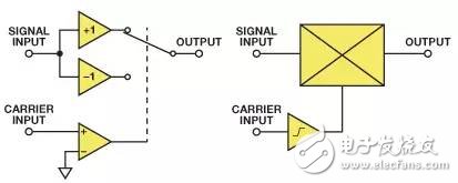
Both designs can form a modulator, yet the switching amplifier architecture (as seen in the AD630 balanced modulator) operates more slowly. High-speed IC modulators usually employ a translinear multiplier (based on Gilbert cells) and feature a limiting amplifier on the carrier path to drive one of the inputs. This limiting amplifier may have high gain, enabling low-level carrier input—or it could have low gain with clean limiting characteristics, necessitating relatively larger carrier inputs for optimal performance.
Despite these differences, we often prefer using a modulator over a multiplier due to several reasons. Multipliers have both inputs as linear, which means any noise or modulated signal from the carrier input gets multiplied by the signal input, reducing the output quality. Meanwhile, the amplitude variations of the modulator’s carrier input can generally be overlooked, though the second-order effects might cause the carrier input’s amplitude noise to influence the output. Best-case modulators minimize this impact, which falls outside the scope of this discussion. A basic modulator model often involves a carrier-driven switch.
An (ideal) open-circuit switch exhibits infinite resistance and zero thermal noise current, whereas a (ideal) closed-circuit switch shows zero resistance and zero thermal noise. Even though the modulator’s switching isn’t ideal, it still generates less internal noise compared to a multiplier. Additionally, designing and manufacturing a high-performance, high-frequency modulator is simpler than constructing a precise multiplier.
Similar to an analog multiplier, the modulator multiplies two signals. Unlike the multiplier, however, the modulator performs non-linear multiplication. When the carrier input’s polarity is positive, the signal input is multiplied by +1; when negative, it’s multiplied by –1. Effectively, the signal is multiplied by a square wave at the carrier frequency.
A square wave with a frequency of ωct can be expressed via the Fourier series' odd harmonics:
\[ K[\cos(\omega_ct) – \frac{1}{3}\cos(3\omega_ct) + \frac{1}{5}\cos(5\omega_ct) – \frac{1}{7}\cos(7\omega_ct) + ...] \]
The series adds up to: [+1, –1/3, +1/5, –1/7 + ...], which equals π/4. Hence, the K value becomes 4/π, making the balanced modulator act as a unity gain amplifier when a positive DC signal is applied to the carrier input.
The carrier amplitude isn’t critical as long as it’s sufficient to drive the limiting amplifier. Thus, the output generated by the modulator driven by the signal Ascos(ωst) and the carrier cos(ωct) is the product of the signal and the square of the carrier:
\[ \frac{2A_s}{\pi}[\cos(\omega_s + \omega_c)t + \cos(\omega_s - \omega_c)t – \frac{1}{3}\{\cos(\omega_s + 3\omega_c)t + \cos(\omega_s - 3\omega_c)t\} + \frac{1}{5}\{\cos(\omega_s + 5\omega_c)t + \cos(\omega_s - 5\omega_c)t\} – \frac{1}{7}\{\cos(\omega_s + 7\omega_c)t + \cos(\omega_s - 7\omega_c)t\} + ...] \]
The output contains the difference between the sum of the frequencies of the following terms and the frequency: all odd harmonics of the signal to the carrier, along with signal and carrier. There’s no even harmonic product in an ideal balanced modulator. However, in a real modulator, the residual offset of the carrier port results in a low-order even harmonic product. In many applications, a low-pass filter (LPF) removes higher harmonic product terms. Since cos(A) = cos(–A), cos(ωm – Nωc)t = cos(Nωc – ωm)t, and there’s no need to worry about "negative" frequencies. After filtering, the modulator output simplifies to:
\[ \frac{2A_s}{\pi}[\cos(\omega_s + \omega_c)t + \cos(\omega_s - \omega_c)t] \]
This matches the multiplier’s output expression, except for slight differences in gain. In practical systems, amplifiers or attenuators normalize the gain, so theoretical gain differences aren’t typically a concern.
In simpler applications, it’s evident that using a modulator is preferable to a multiplier. But how do you define "simple"?
When a modulator acts as a mixer, the signal and carrier inputs are simple sine waves with frequencies f1 and fc, respectively. The unfiltered output includes the frequency sum (f1 + fc) and difference (f1 – fc), along with the odd harmonics of the signal and carrier (f1 + 3fc), (f1 – 3fc), (f1 + 5fc), (f1 – 5fc), (f1 + 7fc), (f1 – 7fc). After LPF filtering, it’s expected to obtain only the fundamental terms (f1 + fc) and (f1 – fc).
However, if (f1 + fc) > (f1 – 3fc), a simple LPF cannot differentiate between the fundamental and harmonic terms because the harmonic term’s frequency falls below a certain fundamental term. This is not a simple scenario and requires further analysis.
Assuming the signal contains a single frequency f1, or if it’s more complex and spans the frequency range f1 to f2, we can analyze the modulator’s output spectrum, as shown in Figure 2. Assuming a perfectly balanced modulator with no signal leakage, carrier leakage, or distortion, the output contains no input terms, carrier terms, or spurious terms. The input is shown in black (or light gray in the output image, even if it doesn't actually exist).
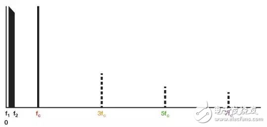
Figure 2 shows the inputs—the signal in the f1 to f2 band and the carrier at frequency fc. The multiplier does not include the following odd carrier harmonics: 1/3 (3fc), 1/5 (5fc), 1/7 (7fc)..., indicated by dashed lines. Note that the fractions 1/3, 1/5, and 1/7 represent amplitude, not frequency.
Figure 3 shows the output of the multiplier or modulator and the LPF with a cutoff frequency of 2fc.
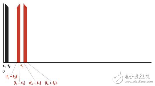
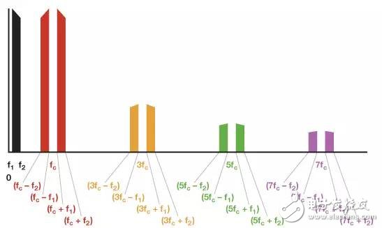
Figure 4 shows the unfiltered modulator output (but does not include harmonic terms above 7fc).
If the signal bands f1 to f2 are within the Nyquist band (DC to fc/2), an LPF with a cutoff frequency higher than 2fc ensures the modulator produces the same output spectrum as the multiplier. The situation becomes more complex if the signal frequency exceeds the Nyquist frequency.
Figure 5 demonstrates what happens when the signal band is just below fc. It’s still possible to separate the harmonic term and the fundamental term, but at this point, an LPF with steep roll-off characteristics is necessary.
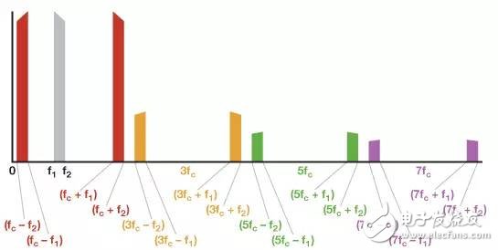
Figure 6 shows that since fc is within the signal passband, the harmonic term (3fc – f1) < (fc + f1), so the fundamental term can no longer be separated from the harmonic term by the LPF. The desired signal must now be selected by a bandpass filter (BPF).
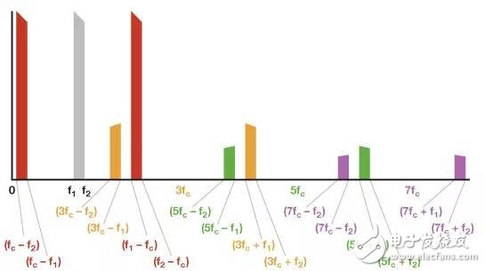
Thus, although modulators outperform linear multipliers in most frequency conversion applications, their harmonics must be considered during system design.
37V Lithium Polymer Battery,Lithium Polymer Battery,3.7 Lithium Polymer Battery,3.7V 4000Mah Lithium Polymer Battery
Langrui Energy (Shenzhen) Co.,Ltd , https://www.langruibattery.com